Full Guide to Freeze Panes, Rows, and Columns in Excel

It is hard to keep track of everything if you are working with plenty of spreadsheet data. To make things easier, you need to freeze panes, rows, and columns in Excel. By doing so, the rows or columns are still visible while you are scrolling through the rest of the worksheet.

Here comes the question. How to freeze panes, rows, and columns in Excel? The content below will illustrate that respectively.

Commonly Used Discord Commands (Like Chat, Bot, and Text)

Discord is widely used for communication. It contains a lot of cool commands. You can carry out multiple operations via the Discord commands.

Read More

How to Freeze Panes in Excel

If you want to freeze panes Excel, you can follow the steps below.

Step 1: Open Excel from your desktop.

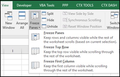
Step 2: Click on the View tab in the top feature area, and then click Freeze Pane option in the Window group.

Step 3: In the pop-up menu, choose an option based on your demand.

Step 4: After that, scroll down to the rest of the worksheet. You can see a dark grey horizontal line on the chosen area that means it is frozen.

How to freeze panes Excel? The above steps have told you. Try them now!

Further reading

To unfreeze the locked content, you can follow these steps.

Step 1: Likewise, click Freeze Panes under the View tab of Excel.

Step 2: In the prompted menu, select Unfreeze Panes.

4 Methods to Troubleshoot the Windows Store Crashing Issue

Are you suffering from the Windows Store crashing issue? If so, this Microsoft Store crashing fix guide comes to use. It offers you top 4 fixes for the error.

Read More

How to Freeze Row in Excel

As mentioned above, you can freeze the first row in Excel via the Freeze Top Row option under the View tab with ease. Hence, we would like to show you how to freeze multiple rows in Excel at here.

Step 1: Launch Excel from your computer.

Step 2: Choose the row below the last row to freeze. To be specific, if you want to free the top 3 rows, you should choose cell A4 or the whole row 4.

Step 3: Click Freeze Panes > Freeze Panes under the View tab.

With the above steps, Excel freeze panes in a flash.

How to Fix and Increase the Outlook File Size Limit

Have you encountered the file sending failure because of Outlook file size limit? If you have, you can solve the issue with this tutorial.

Read More

How to Freeze Columns in Excel

To freeze columns in Excel, you can follow these steps.

Step 1: Choose the column to the right of the last column that you would like to freeze. For instance, to freeze the first 5 columns, you should choose the whole column F or cell F1.

Step 2: After selecting the target content, click Freeze Panes > Freeze Pane.

Step 3: After that, the selected area will be frozen.

If you don’t know how Excel freeze panes, check the above content right now!

Bonus Tip: What to Do When Freeze Panes Not Working

Sometimes, you may find that the Freeze Panes Excel option is greyed out (disabled). It is probably that you are in the cell editing mode. In this case, you should press Enter or Esc key to exit the cell editing mode.

When the worksheet is protected, the Freeze Panes not working error occurs too. For that, you need to unprotect the Excel sheet by right-clicking the sheet and choose Unprotect Sheet.